1 Calculus with Vectors and Matrices Here are two rules that will - PDF document
Mathematical Tools for Neuroscience (NEU 314) Princeton University, Spring 2016 Jonathan Pillow Lecture 10: Least Squares Squares 1 Calculus with Vectors and Matrices Here are two rules that will help us out with the derivations that come
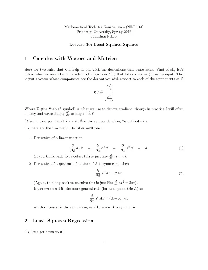
Mathematical Tools for Neuroscience (NEU 314) Princeton University, Spring 2016 Jonathan Pillow Lecture 10: Least Squares Squares 1 Calculus with Vectors and Matrices Here are two rules that will help us out with the derivations that come later. First of all, let’s define what we mean by the gradient of a function f ( � x ) that takes a vector ( � x ) as its input. This is just a vector whose components are the derivatives with respect to each of the components of � x : ∂f ∂x 1 . ∇ f � . . ∂f ∂x d Where ∇ (the “nabla” symbol) is what we use to denote gradient, though in practice I will often be lazy and write simply d f ∂ x or maybe x f . d� ∂� (Also, in case you didn’t know it, � is the symbol denoting “is defined as”). Ok, here are the two useful identities we’ll need: 1. Derivative of a linear function: ∂ ∂ ∂ a ⊤ � x ⊤ � x � a · � x = x � x = x � a = � a (1) ∂� ∂� ∂� d (If you think back to calculus, this is just like dx ax = a ). 2. Derivative of a quadratic function: if A is symmetric, then ∂ x ⊤ A� x � x = 2 A� x (2) ∂� dx ax 2 = 2 ax ). d (Again, thinking back to calculus this is just like If you ever need it, the more general rule (for non-symmetric A ) is: ∂ x ⊤ A� x = ( A + A ⊤ ) � x � x, ∂� which of course is the same thing as 2 A� x when A is symmetric. 2 Least Squares Regression Ok, let’s get down to it! 1
Suppose someone hands you a stack of N vectors, { � x N } , each of dimension d , and an asso- x 1 , . . . � ciated scalar observation { y 1 , . . . , y N } . You’d like to estimate a linear function that allows us to predict y from � x as well as possible: w ⊤ � y i ≈ � x i for some weight vector � w . Specifically, we’d like to minimize the squared prediction error, so we’d like to find the � w that minimizes N � w ) 2 squared error = ( y i − � x i · � (3) i =1 We’re going to write this as a vector equation to make it easier to derive the solution. Let Y be a vector composed of the stacked observations { y i } , and let X be the vector whose rows are the vectors { � x i } (which is known as the design matrix ): y 1 — x 1 � — . . . . Y = X = . . y N — x N � — Then we can rewrite the squared error given above as the squared vector norm of the residual error between Y and X � w : w || 2 squared error = || Y − X � (4) 2.1 Derivation #1: calculus We can call our first derivation of the solution (i.e., the � w vector that minimizes the squared error defined above) the “straightforward calculus” derivation. We will differentiate the error with respect to � w , set it equal to zero (i.e., implying we have a local optimum of the error), and solve for w . All we’re going to need is some algebra for pushing around terms in the error, and the vector � calculus identities we put at the top. Let’s go! ∂ w SE = ∂ w ) ⊤ ( Y − X � w ( Y − X � w ) (5) ∂ � ∂ � = ∂ � w ⊤ X ⊤ + � � Y ⊤ Y − 2 � w ⊤ X ⊤ XY (6) ∂ � w = − 2 X ⊤ Y + 2 X ⊤ X � w = 0 . (7) We can then solve this for � w as follows: X ⊤ X � w = X ⊤ Y (8) w = ( X ⊤ X ) − 1 X ⊤ Y = ⇒ (9) � 2
Easy, right? (Note: we’re assuming that X ⊤ X is full rank so that its inverse exists, implying that N > d and the rows are not all linearly dependent with each other. ) 2.2 Derivation #2: orthogonality Our second derivation is even easier, and it has the added advantage that it gives us some geomtrix insight. Let’s think about the design matrix X in terms of its d columns instead of its N rows. Let { X j } denote the j ′ th column, i.e., X = X 1 · · · X d (10) The columns of X span a d -dimensional subspace within the larger N -dimensional vector space that contains the vector Y . Generally Y does not lie exactly within this subspace. Least squares regression is therefore trying to find the linear combination of these vectors, X � w , that gets as close to possible to Y . What we know about the optimal linear combination is that it corresponds to dropping a line down from Y to the subspace spanned by { X 1 , . . . X D } at a right angle. In other words, the error vector ( Y − X � w ) (also known as the residual error ) should be orthogonal to every column of X : ( Y − X � w ) · X j = 0 , (11) for all j columns. Written as a matrix equation this means: w ) ⊤ X = � ( Y − X � 0 (12) where � 0 is d -component vector of zeros. We should quickly be able to see that solving this for � w gives us the solution we were looking for: X ⊤ ( Y − X � w ) = X ⊤ Y − X ⊤ X � w = 0 (13) ( X ⊤ X ) � w = X ⊤ Y = ⇒ (14) w = ( X ⊤ X ) − 1 X ⊤ Y. = ⇒ � (15) So to summarize: the requirement that the residual errors between Y and X � w be orthogonal to the columns of X was all we needed to derive the optimal � w ! 3 Derivation for PCA In the last lecture on PCA we showed that if we restricted ourselves to considering eigenvectors of the X ⊤ X , then the eigenvector with largest eigenvalue captured the largest projected-sum-of- 3
squares of the vectors contained in X . But we didn’t show that eigenvectors themselves correspond to optima of the PCA loss function. To recap briefly, we want to find the maximum of v ⊤ C� � v, where C = X ⊤ X is the (scaled) covariance of zero-centered data vectors X , subject to the constraint v ⊤ � that � v is a unit vector ( � v = 1). We can solve this kind of optimization problem using the method of Lagrange multipliers. The basic idea is that we minimize a function that is our original function plus a lagrange multiplier λ times an expression that is zero when our constraint is satisfied. For this problem we can define the Lagrangian: v ⊤ C� v ⊤ � L = � v + λ ( � v − 1) . (16) We will want solutions for which ∂ v L = 0 (17) ∂� ∂ ∂λ L = 0 . (18) Note that the second of these is satisfied if and only if � v is a unit vector (which is reassuring). The first equation gives us: ∂ v L = ∂ v ⊤ � v � vC� v + λ ( � v − 1) = 2 C� v − 2 λ� v = 0 , (19) ∂� ∂� which implies v = − λ� (20) C� v. What is this? It’s the eigenvector equation! This implies that the derivative of the Lagrangian is zero when � v is an eigenvector of C . So this establishes, combined with the argument from last week, that the unit vector that captures the greatest squared projection of the raw data is the top eigenvector of C . 4
Recommend
More recommend
Explore More Topics
Stay informed with curated content and fresh updates.
