1 12 Exploratory Factor Analysis (EFA): Brief Overview with - - PDF document

1

12 Exploratory Factor Analysis (EFA): Brief Overview with Illustrations Topics

• 1. Logic of EFA
• 2. Formative vs Reflective Models, and Principal Component Analysis (PCA) vs Exploratory Factor Analysis (EFA)
• 3. EFA Steps, Components, and Concepts
• 4. Example 1: Autonomy Support and Student Ratings of Instruction
• 5. Example 2: Employment Thoughts Data
• 6. Example 3: Doctoral Student Efficacy and Anxiety toward the Dissertation Process
• 7. Example 4: Parenting Stress and Coping in Difficult Parenting Situations
• 8. Reading Factor Analysis Tables
• 8. Sample Size for EFA (to be added)
• 1. Logic of EFA

EFA is designed to determine whether a set of variables can be reduced to a smaller number of factors due to clustering

• r correlation among variable scores. If two variables correlate highly, for example, it is possible they represent the

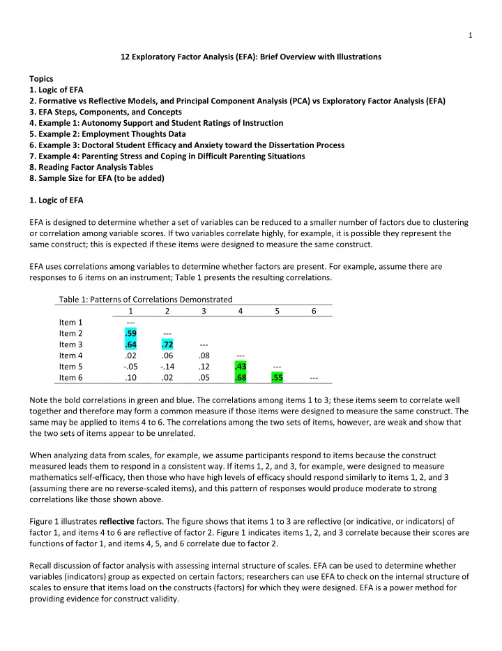
same construct; this is expected if these items were designed to measure the same construct. EFA uses correlations among variables to determine whether factors are present. For example, assume there are responses to 6 items on an instrument; Table 1 presents the resulting correlations. Table 1: Patterns of Correlations Demonstrated 1 2 3 4 5 6 Item 1

• Item 2

.59

• Item 3

.64 .72

• Item 4

.02 .06 .08

• Item 5
• .05
• .14

.12 .43

• Item 6

.10 .02 .05 .68 .55

• Note the bold correlations in green and blue. The correlations among items 1 to 3; these items seem to correlate well

together and therefore may form a common measure if those items were designed to measure the same construct. The same may be applied to items 4 to 6. The correlations among the two sets of items, however, are weak and show that the two sets of items appear to be unrelated. When analyzing data from scales, for example, we assume participants respond to items because the construct measured leads them to respond in a consistent way. If items 1, 2, and 3, for example, were designed to measure mathematics self-efficacy, then those who have high levels of efficacy should respond similarly to items 1, 2, and 3 (assuming there are no reverse-scaled items), and this pattern of responses would produce moderate to strong correlations like those shown above. Figure 1 illustrates reflective factors. The figure shows that items 1 to 3 are reflective (or indicative, or indicators) of factor 1, and items 4 to 6 are reflective of factor 2. Figure 1 indicates items 1, 2, and 3 correlate because their scores are functions of factor 1, and items 4, 5, and 6 correlate due to factor 2. Recall discussion of factor analysis with assessing internal structure of scales. EFA can be used to determine whether variables (indicators) group as expected on certain factors; researchers can use EFA to check on the internal structure of scales to ensure that items load on the constructs (factors) for which they were designed. EFA is a power method for providing evidence for construct validity.

2

• 2. Formative vs Reflective Models, and Principal Component Analysis (PCA) vs Exploratory Factor Analysis (EFA)

Many argue that factor analysis and principal component analysis are essentially the same, and it is true that they often produce similar results. Conceptually, however, the two are very different. PCA is designed to produce “a linear combination of variables; Factor Analysis is a measurement model of a latent variable” (Karen, 2018). With PCA, the model for a component is C = b1 X1 + b2 X2 + b3 X3 … where C is the component, b are the coefficients, and X are the variables or items. With EFA, the model is X1 = b1 F1 + b2 F2 + b3 F3 + … + u1 where X is the indicator or item, b are the coefficients, F are the factors, and u is the error term for each X. An EFA model is illustrated in Figure 1 and a PCA model is illustrated in Figure 2. EFA is for reflective constructs and PCA is for formative constructions. Figure 1: Reflective Model with Two Factors Figure 2: Formative Model with Two Components Reflective models assume that the factor is the causal agent leading to scores obtained for the indicators; the factor predicts or causes variation in the indicators, so the factor is the independent variable and the indicators are the dependent variables. With this model one assumes that the factor exists independent of the indicators; we use indicators to help us measure the factor. The factor is the causal agent and results in variation observed in the

3

• indicators. Example: The greater your math self-efficacy (factor), the (a) more time you spend on difficult problems

(indicator), the (b) more interest you have in math (indicator), and the (c) more confidence you have with math problems (indicator). Formative models represent a different causal assumption compared with reflective models. With formative models, the indicators are predictors or causal agents for variation in the component. Indicators are the independent variables and the component is the dependent variable. It is also possible to view this model not as cause and effect, but simply as a mathematical structure such that the indicators are used to form a composite variable called a component. In either view, the component is formed by combining indicators; this suggests the component may not exist independent of the indicators, although that is not the case in every situation (e.g., see cyber-harassment example below – victim experience exists independent of the indicators). Example: The greater one’s (a) wealth (indicator), (b) education (indicator), and (c) occupational prestige (indicator), the greater one’s socio-economic status (SES; component). Coltman et al (2008) explain that with reflective models we expect to see strong correlations among items and thus high internal consistency for each factor; with formative models items may be independent and uncorrelated since the component is a composite; there is no need for items to correlate (although if there are correlations, the items must correlate positively otherwise reverse scoring is needed because failure to reverse score means items are both adding and subjecting from the composite variable score). Internal consistency is expected and assessed with reflective models, but not necessary for formative models. Example of Reflective and Formative Models: Cyber-harassment Cyberbullying exists as both reflective and formative models. Suppose we ask the following three questions.

• 1. Visual harassment – electronically posting images or videos with the intent to embarrass, threaten, intimidate, offend,

manipulate, harass, or otherwise make someone experience negative reactions.

• 1V. How many times has this happened to you in

the past 3 years?

• 0. Never
• 1. 1 time
• 2. 2 times
• 3. 3 times
• 4. 4 or more times
• 1B. How many times have you done this to

someone else in the past 3 years?

• 0. Never
• 1. 1 time
• 2. 2 times
• 3. 3 times
• 4. 4 or more times
• 2. Written harassment – electronically posting written message with the intent to embarrass, threaten, intimidate,
• ffend, manipulate, harass, or otherwise make someone experience negative reactions.
• 2V. How many times has this happened to you in

the past 3 years?

• 0. Never
• 1. 1 time
• 2. 2 times
• 3. 3 times
• 4. 4 or more times
• 2B. How many times have you done this to

someone else in the past 3 years?

• 0. Never
• 1. 1 time
• 2. 2 times
• 3. 3 times
• 4. 4 or more times

4

• 3. Spoken/Verbal harassment – to speak or leave a spoken message electronically with the intent to embarrass,

threaten, intimidate, offend, manipulate, harass, or otherwise make someone experience negative reactions.

• 3V. How many times has this happened to you in

the past 3 years?

• 0. Never
• 1. 1 time
• 2. 2 times
• 3. 3 times
• 4. 4 or more times
• 3B. How many times have you done this to

someone else in the past 3 years?

• 0. Never
• 1. 1 time
• 2. 2 times
• 3. 3 times
• 4. 4 or more times

Items 1V, 2V, and 3V are indicators for victims cyer-harassment, and items 1B, 2B, and 3B are indicators of cyber- harassment bullying behavior. The wording of items 1V, 2V, and 3V make clear the experience of cyber-harassment was thrust upon the vicitm, and the wording of items 1B, 2B, and 3B make clear these harassment behaviors were caused by the bully. The theoretical model for cyber-harassment is shown in Figure 3. Figure 3: Formative and Reflective Models for Cyber-harassment Vicitms are subjected to harassment activities. These experiences are directed toward them; they are not the perpetrator of these actions, so the causal links in Figure 3 must flow from item to componet. This is an example that would be suitable for PCA – a composite indicator of victim experience. Bullies, on the other hand, initiate and perpetrate cyber-harassing behaviors. These behaviors and actions emanate from the bully – the bully is the causal agent of these behaviors. Given this, the links flow from from factor to item. This is an exampel that would be suitable for EFA – a theoretical measurment model for the bully behavior.

• 3. EFA Steps, Components, and Concepts

EFA assumes variables are ordinal (~5 or more categories), interval, or ratio. EFA software is typically not designed for nominal or categorical variables. Variables must be able to form a correlation (or covariance) matrix for analysis. (a) Initial Extraction With the initial extraction we obtain estimates of amount of variance each factor predicts among all model indicators. We expect this to be high, usually 60% or more. Eigenvalues are reported; these indicate the amount of factor variance attributed to each factor.

5

Communalities are also reported; these are R2 values that indicate the proportion of variance in each indicator that is predicted by the factors. Items with low communalities are not predicted well by factors and perhaps should be

• removed. They tend to show low loadings with both before and after rotation.

An extraction method must be selected. Principal Axis Factoring is commonly used and will be recommended here. Other options exist and often results are similar. We can learn whether the correlation matrix among indicators is suitable for EFA by examing Bartlett’s test of sphericity and Kaiser-Meyer-Olkin (KMO) measure of sampling adequacy. Note that usually one analzes the correlation matrix because the covariance matrix can present difficult to interpret loading if indicator variances greatly differ. (b) Determine Number of Factors to Retain Examine results of the initial extraction to help determine how many factors should be retained in the measurement

• model. This can be done several ways:
• Theoretical Model – if scale developed for three factors, then one should see three factors
• Scree Plot – look for elbow in screen plot (a sharp turn to the right) to determine number of factors
• Eigenvalues Size – a default option is to select the number of factors with eigenvalues greater than 1.00
• Percentage Explained – keep number of factors that account for 70% or 80% of item variance
• Parallel Analysis – estimate eigenvalues size expected by chance and select only those eigenvalues larger than

what would be expected by chance (c) Factor Rotation and Interpretation The goal with this step is to simplify the factor loadings to make factor interpretation easier. A simple structure is sought; this means indicators load high on one factor and low on other factors. Orthogonal rotation means the factors are uncorrelated. This is rarely a reasonable assumption so I don’t recommend

• rthogal rotation options (e.g, Varimax).

Oblique rotation means factors are correlated and this is usually reasonable. Oblimin is the oblique option provided in my version of SPSS. Examine factor loadings to determine factor composition and description; factor loadings are used to name factors.

• 4. Example 1: Autonomy Support and Student Ratings of Instruction

Student Ratings Data http://www.bwgriffin.com/gsu/courses/edur9131/2018spr-content/12-factor-analysis/studentratingsdata.sav Two constructs of interest: Construct 1: Autonomy Support

• 24. The instructor was willing to negotiate course requirements with students.
• 25. Students had some choice in course requirements or activities that would affect their grade.
• 26. The instructor made changes to course requirements or activities as a result of student comments or

concerns.

6

Construct 2: Student Ratings of Instructor and Course

• 5. The instructor presented the material in a clear and understandable manner.
• 6. Course materials were well prepared and organized.
• 8. The instructor made students feel welcome in seeking help/advice in or outside of class.
• 9. The content of this course is useful, worthwhile, or relevant to you.
• 10. Methods of evaluating student work were fair and appropriate.
• 13. The instructor gave students useful/helpful feedback on work.
• 29. Overall, how would you rate this course?
• 30. Overall, how would you rate this instructor?

The purpose of this EFA is to assess the internal structure of these two scales (construct validity check). Ideally two distinct factors would emerge, one for autonomy support (only items 24, 25, and 26 load on this factor), and one for student ratings (all other variables should load on this factor). We hope to see weak loadings across factors for variables that were not designed to measure that construct, i.e., hope to find simple structure. SPSS Factor Analysis Commands Before proceeding to EFA, first check the correlation matrix among variables to ensure things look appropriate. Always check that items are reversed scored as needed, and that reversed items are included instead of the original un-reversed items. Analyze -> Data Reduction (or Dimension Reduction) -> Factor Move items identified above into the Variables box. Items include the following items: v5, v6, v8, v9, v10, v13, v29, v30, v24, v25, v26 Descriptives -> Check boxes noted below

• Univariate Descriptives
• Initial Solution
• Coefficients
• Determinant
• KMO and Bartlett’s test of spherecity

7

Extraction –> Method = Principal Axis Factoring (don't use Principal Component Analysis, that is different from factor analysis) Analyze = Correlation Matrix Display = Unrotated factor solution Display = Scree Plot Eigenvalue over = 1

8

Rotation -> Method = Direct Oblimin (0) – this is an oblique rotated solution Display = Rotated Solution Display = Loading Plots Options -> Coefficient Display Format = Sorted by size (this will sort loadings by size, easier to see results) SPSS Factor Analysis Results What do the results tell us? Do we have two factors? Do the items load on the factors as hoped? Do the results support the internal structure (hence construct validity) of these two scales? Note – add determinant; it should not be 0.00 otherwise there will be difficulty with computations in EFA.

9

(a) KMO and Bartlett Tests The KMO test assesses whether the pattern of correlations in the correlation matrix suggest natural groupings or whether groupings of items appear weak. Recall the correlation matrix at the outset of this presentation – the correlations there formed two groupings highlighted in green and blue. That correlation matrix would work well for factor analysis. KMO should be closer to 1.00. KMO value interpretation:

• below .5 don’t attempt EFA,
• .5 and .6 are awful,
• .6 and .7 are acceptable but not good;
• .7 and .8 are good;
• .8 to .9 very good, and above
• .9+ super-duper good.

KMO should be >.6, but ideally .8 and above Bartlett’s test assesses whether the correlation is an identify matrix – this means the correlations between all items is 0.00 (no correlation). If there is no correlation, then EFA is not possible. We want Bartlett’s test to be significant because rejecting the null means there are correlations among variables and EFA is suitable. Bartlett should be significant at .05 level (i.e., Sig < .05) Both tests suggest these data are appropriate for EFA. The correlation matrix below illustrates what Bartlett’s test assesses as the null hypothesis. If the correlation matrix looked like this, EFA would not be possible. Table 2: Identify Matrix – No correlations Among Items 1 2 3 4 5 6 Item 1 1.00 .00 .00 .00 .00 .00 Item 2 .00 1.00 .00 .00 .00 .00 Item 3 .00 .00 1.00 .00 .00 .00 Item 4 .00 .00 .00 1.00 .00 .00 Item 5 .00 .00 .00 .00 1.00 .00 Item 6 .00 .00 .00 .00 .00 1.00 (b) Communalities (symbol h2) The table below shows communalities. The Initial column are communality estimates before factor extraction and therefore not of interest for interpretation purposes. These are determined by the R2 obtained in regression where one variable is modeled by all others (e.g., V5 treated as a DV and all others – V6 through V30 – are the IVs predicting V5).

10

The Extraction column shows communities for each variable after extraction of the two factors that were retained (see below). These numbers can be interpreted as R2 values in regression – the proportion of variance in each variable explained or predicted by the extracted factors. For example, the communality for V5 is .88 which means the two factors extracted predict about 88% of the variance in V5. Our hope is that communalities after extraction are high for each variable. If the communality is low, this means the factors extracted are unable to predict variation in that variable, so it probably does not fit the measurement model examined, i.e., it does not help us measure any factors. Technically h2 is the sum of the squared factor loadings for the variable. (c) Variance Explained The Factor column is the number of possible factors which always equals the number of variables included in the EFA. Not all 11 factors in this example will be retained.

11

The Eigenvalue columns include Total, % of Variance, and Cumulative %. Since the correlation matrix was analyzed, each factor as a variance of 1.00, and since there are 11 factors, the Total column, if summed, would equal 11. The total column shows that two eigenvalues exceeded 1.00, Factor 1 = 7.415 and Factor 2 = 2.306. This means factor 1’s variance was 7.415 and factor 2’s variance was 2.306. Of the total variance possible, 11 in this case since there are 11 variables, Factor 1 accounted for 7.415 / 11 = 0.674 or 67.4% of the total variance in factors. Factor 2 accounted for 2.306 / 11 = .209 or 20.9% of the total variance. Together, Factors 1 and 2 accounted for 85.507% of the common variance in factors after extraction of the two factors. Notice that in the columns labeled Extraction of Sums of Squared Loadings there are only two rows – this set of columns presents only information for the number of factors extracted. The Rotation Total column is the total common variance for the retained factors. (d) Determining Number of Factors to Extract Identified above were several approaches to determining the number of factors to extract. Each will be considered below.

• d1. Theoretical Model

Two scales were included with these data, Autonomy Support and Student Ratings, so there should be two factors identified.

• d2. Scree Plot

This plot shows eigenvalues by number of factors. The idea is that clear factors will form a vertical line, and non-factors will form a horizontal line. Where these join forms an elbow or right bend, and that is the area used to make a cut between which factors to retain and which to drop. In the graph below a red line has been added separating the vertical and horizontal pattenrs – factors above the red line should be retained. In this case, two factors are identified. Origin of scree – rubble located at bottom of mountains.

12

• d3. Eigenvalues Size

Another option is to retain factors with eigenvalues that exceed a pre-specified level, which is often defined as 1.00. Using this criterion, two factors had eigenvalues greater than 1.00, so two factors should be retained. This is the default in SPSS and the reason two factors were extracted in this first run of EFA. If we believe the number of factors extracted by eigenvalue size is incorrect, we can easily specify the number of factors to retain in the the Factor Analysis: Extracton screen by placing that number in the box below indicated by the red arrow.

• d4. Percentage Explained

Another approach is the retain the number of factors that account for 70% or 80% of the total factor variance. In this example, the two factors accounted for 88.365% of the factor variance, so this suggests two factors should be retained.

• d5. Parallel Analysis

Note – this site seems to produce invalid scores – compare with other estimates (e.g. Stata) Parallel analysis estimates the size of factor eigenvalues from a large number randomly generated correlation matrices. The logic: randomly generated correlations will lead to purely random eigenvalues, so compare the eigenvalues

• btained from real data against those generated from random data; if the real eigenvalues are larger than their random

13

counterparts, then those must be real factors; if eigenvalues from real data are less than eigenvalues from random data, then those must be random factors embedded in the real data. Parallel analysis eigenvalues can be obtained from this site; results are shown below. https://analytics.gonzaga.edu/parallelengine/ Note – discuss screenshot above in class. The parallel analysis shows that 2 factors should be retained. All approaches considered above – theorectical mode, scree plot, eigenvalue size, percent explained, and parallel analysis – suggest that 2 factors should be retained.

14

(e) Initial Factor Loadings The Factor Matrix (pattern matrix) table contains the unrotated factor loadings, the correlations between variables and

• factors. This table can provide some ideas about which variables load on which factors. Highlighted in red are the

highest loadings for each factor. It seems Factor 1 is composed of the Student Ratings items, and Factor 2 the three Autonomy Support items. These loadings are easy to read and show clearly that Factor 1 represent student ratings and Factor 2 represents autonomy support. In cases like this, factor rotation to simplify interpretation is not needed because the factors are easy to read. Sometimes loadings are not so easy to read, and factor rotation can help clarify the picture. The communality for each variable can be found by squaring and adding the loadings reported in the Factor Matrix table (note – I think this does not work for rotated tables, check this). For example, V30 loadings squared and summed are .9622 + -.1572 = .95, the same value reported above in the communalities table. Note: The unrotated Factor Matrix is both factor coefficient and factor correlation (i.e., both pattern and structure). For

• rthogonal rotations, both pattern and structure matrices, described below, are the same.

(e) Factor Rotation and Interpretation Recall that an oblique rotation was requested (oblimin) which allows factors to correlate. Rotated factor loadings are shown below in both the Pattern and Structure Matrices. Pattern matrix – Coefficients for linear combinations of variables (factor coefficients used to reproduce variable scores, predict variable scores, like regression coefficients). Most use this matrix for interpretation of factors; usually both pattern and structure provide similar interpretations for factors. Structure matrix – Correlations between factors and variables after oblique rotation Rotation – Redistribute variable loadings on each factor in such a way to help produce a simple structure to make interpretation easier. Common rotation options are briefly described below. Orthogonal Rotations (Factors Uncorrelated)

• Varimax: Minimizes the number of variables that have high loadings on each factor identified.
• Quartimax: Minimizes number of factors with high loadings with variables.

15

• Equamax: Combination of both varimax and quartimax.
• I do not recommend use of any Orthogonal rotation methods since these may artificially discard useful

information about how factors are related. Oblique Rotations (Factors Correlated)

• Oblimin (or Direct Oblimin): The degree of correlation between factors is controlled by delta. In SPSS the

default is 0. Negative values of delta result in weaker factor correlations and positive values result in stronger factor correlations. It is not clear of the potential range for delta, but 0 appears to be a mid-range value in terms of producing factor correlations. The upper value for delta is 0.80; I am uncertain about the lowest value of delta. Values below -4 tend to produce factors that are nearly uncorrelated.

• Promax: Another orthogonal rotation method – often presented as quicker than Oblimin, but that is not a

concern for those who use computers to rotate factors.

• I recommend using Oblique rotation methods, and do not have a recommend for which, oblimin or promax,

to use. If using oblimin, unless there is reason to change delta, leave it at 0.00. The Pattern Matrix presents the pattern loadings, or coefficients, linking each factor with each variable. The pattern matrix is often used to interpret factors. Results shown in the pattern matrix demonstrate what is known as simple structure – high loadings on one factor and low loadings on the other factor. Item V29, for example, has a high loading

• n Factor 1 (.980), but a low loading on Factor 2 (-.048), so this indicates V29 is aligned closely with Factor 1 but not with

Factor 2. Interpretation of the pattern matrix is the process of identifying which variables, or scale items, load well and poorly on a factor. Those items with high loadings must be considered when naming a factor. Factor 1 in the current pattern is dominated by the Student Ratings variables, shown below. Factor 1 = Student Ratings

• 5. The instructor presented the material in a clear and understandable manner.
• 6. Course materials were well prepared and organized.
• 8. The instructor made students feel welcome in seeking help/advice in or outside of class.
• 9. The content of this course is useful, worthwhile, or relevant to you.
• 10. Methods of evaluating student work were fair and appropriate.
• 13. The instructor gave students useful/helpful feedback on work.

16

• 29. Overall, how would you rate this course?
• 30. Overall, how would you rate this instructor?

Factor 2 has a very simple structure – Autonomy Support items, see below, load very well on Factor 2, and Student Ratings items show almost no loading on Factor 2. Factor 2 = Autonomy Support

• 24. The instructor was willing to negotiate course requirements with students.
• 25. Students had some choice in course requirements or activities that would affect their grade.
• 26. The instructor made changes to course requirements or activities as a result of student comments or

concerns. The Structure Matrix shows the structure loadings, or the correlation between each variable and factor. This table can also be used to interpret factors, and the results are the same as shown in the Pattern Matrix – items V26, V25, and V24 load best on Factor 2, so Factor 2 is the Autonomy Support factor. Factor Correlations The Factor Correlation Matrix table shows the correlation between Factor 1 (which I named Student Ratings) and Factor 2 (which I named Autonomy Support). It appears that autonomy support correlates .339 with Student Ratings. This correlation was obtained with the oblimin delta = 0.00. Below are estimates of factor correlations between student ratings and autonomy support for different values of

• blimin delta.

Oblimin Delta Correlation between Factors 1 and 2 Oblimin Delta Correlation between Factors 1 and 2 .8 .765

• .5

.274 .5 .550

• .8

.252 .2 .392

• 1

.240 .339

• 2

.195

• .2

.306

• 4

.138 With delta = -500, the correlation was .005. It appears that as delta approaches -∞ the factor correlation approaches 0.00. As a comparison, I computed mean composite scores for both autonomy and student ratings. The correlation obtained from the composite scores was .367 which is close to the value or .339 provided when delta = 0.00. Factor Plots The plot below shows how the items cluster in space for Factors 1 and 2. This clustering demonstrates clear separation thereby confirming the two-factor solution.

17

Figure x: Factor Plot with Unrotated Factors Figure x: Factor Plot with Rotated Factors (Oblimin, delta = 0) Note - Factor Scores, to be added; discuss possible use, see Kootsra Exploratory Factor Analysis p. 8 for uses. Note – add goodness of fit expanded discussion Briefly, goodness of fit of this two factor EFA?

• KMO = .874 (very good)
• Percent variable predicted = 85.5%
• Communalities = range from low of .749 to high of .95
• Factor pattern = clear factors
• Reproduced correlation matrix = note, add discussion of deviance, how many residual >.05?

18

• 5. Example 2: Employment Thoughts Data

Some of you completed questionnaire twice for this course. The items were selected from Menon (2001) and were designed to measure three employment related constructs. Responses to each item scaled from Strongly Disagree (1) to Strongly Agree (6). Perceived Control Q1: I can influence the way work is done in my department Q2: I can influence decisions taken in my department Q3: I have the authority to make decisions at work Goal Internalization Q4: I am inspired by what we are trying to achieve as an organization Q5: I am inspired by the goals of the organization Q6: I am enthusiastic about working toward the organization’s objectives Perceived Competence Q7: I have the capabilities required to do my job well Q8: I have the skills and abilities to do my job well Q9: I have the competence to work effectively SPSS data file link (can be found in Reliability section on course web page): http://www.bwgriffin.com/gsu/courses/edur9131/2018spr-content/06-reliability/06-EDUR9131-EmploymentThoughts- Merged.sav

• 6. Example 3: Doctoral Student Efficacy and Anxiety toward the Dissertation Process

(Illustrate analysis in class) Efficacy and anxiety toward the dissertation process. Odd items measure efficacy and even items measure anxiety. Data 2: http://www.bwgriffin.com/gsu/courses/edur9131/temp/alphadata.sav Alpha Data Questions: http://www.bwgriffin.com/gsu/courses/edur9131/activities/Assignment_6_internal_consistency_data.pdf

• 7. Example 4: Parenting Stress and Coping in Difficult Parenting Situations

Szymańska A, Dobrenko KA. (2017) The ways parents cope with stress in difficult parenting situations: the structural equation modeling approach. PeerJ 5:e3384 https://peerj.com/articles/3384/ Szymańska and Dobrenko (2017) present the following figure showing relations among a number of constructs. They also present their data in an SPSS file, which is linked below. https://dfzljdn9uc3pi.cloudfront.net/2017/3384/1/base_for_review_stress.sav I have also saved these data to the course web site, linked below. http://www.bwgriffin.com/gsu/courses/edur9131/2018spr-content/12-factor-analysis/12-2017-Szymanska-data.sav

19

While EFA cannot be used to assess the structural relations among constructs in the model below, it can be used to assess whether the measurement model – the factors and their loadings – are similar to those shown in the figure. The variables used to measure each construct are identified above. Discrepancy = rozb1 to rozb6 Representation = r1 to r8 Cognitive Distancing = S2 s3 s4 Help Seeking = S1 s5 s6 Difficulty = tr1 to tr8 Pressure = s7 s8 s9 Withdrawal = s10 to s15 EFA with all variables entered. According to their model, there should be 7 overall factors, or possible 9 if Representation and Discrepancy both divide into 2 sub-factors as shown in the figure.

20

Data entered in EFA Descriptive sought Extraction method Rotation approach

21

Options – sort results by size and exclude values of .30 or less in absolute value SPSS Results Descriptive show n = 258 KMO and Bartlett – both are very good Variance Explained – total of 37 variables entered, 8 factors with eigenvalues greater than 8, so SPSS extracts 8 factors by default

22

How many factors to retain? 7-1. Theoretical Model As noted, there are 7 overall factors, and maybe 9 if two factor sub-divide into two factors each. 7-2. Scree Plot The scree plot is not clear, but maybe 8 according to the line I drew below.

23

7-3. Eigenvalues Size There are 8 factors with eigenvalues larger than 1. 7-4. Percentage Explained Eight factors explain 75.8% of variance, which hits the mark of 70% to 80% variance expalined. 7-5. Parallel Analysis (Note, this page seems to provide inaccurate parallel analysis results – compare against Stata) https://analytics.gonzaga.edu/parallelengine/

24

The parallel analysis shows that more than 13 factors should be retained, so this does not appear to be a useful assesment. Overall most approaches to assessing factor extraction seem to suggest 8 factors, so we will proceed with 8 factors. Pattern Matrix – overall the results are very good (see below). In most cases each factor has loadings that are unique to that factor (simple structure) except for Difficulty which is correlated to Representation (child’s task). Given the number

• f items (n = 37) and the number of constructs to measure (7 or 9), this EFA did well recreating the factor structure.

25

26

Out of curiosity, I re-ran the EFA but specified 9 factors should be extracted. Results are shown below. The EFA almost perfectly reproduced the factor structure expected for the questionnaire – this is a strong indication that the 9-factor extraction is the appropriate solution. Overall their measures of these 9 constructs worked very well to independently assess these 9 constructs. These are excellent results. Pattern Structure matrix on next page.

27

28

• 8. Reading Factor Analysis Tables

How to select best items using EFA results. http://www.bwgriffin.com/gsu/courses/edur9131/2018spr-content/12-factor-analysis/12-2004-Tschannen-principal- efficacy.pdf

29

http://www.bwgriffin.com/gsu/courses/edur9131/2018spr-content/12-factor-analysis/12-2008-Thomas-science- selfefficacy.pdf Complete wording of items presented in the appendix.

30

• 8. Sample Size for EFA

See Costello and Osborne (2005) for discussion of sample size. to be added References Coltman, T., Devinney, T.M., Midgley, D.F., & Venaik, S. (2008). Formative versus reflective measurement models: Two applications of formative measurement. Journal of Business Research, 61, 1250-1262, Floyd, F. & Widaman, K.F. (1995). Factor analysis in the development and refinement of clinical assessment instruments. Psychological Assessment, 3, 286-299. Karen, (2018). “The Fundamental Difference Between Principal Component Analysis and Factor Analysis.” Retried 13 April 2018 from: https://www.theanalysisfactor.com/the-fundamental-difference-between-principal-component- analysis-and-factor-analysis/ Costello, Anna B. & Jason Osborne (2005). Best practices in exploratory factor analysis: four recommendations for getting the most from your analysis. Practical Assessment Research & Evaluation, 10(7). Available online: http://pareonline.net/getvn.asp?v=10&n=7