1 1 MILES SPAN MINIMUM SPANNING TREES Important: Before reading - PDF document
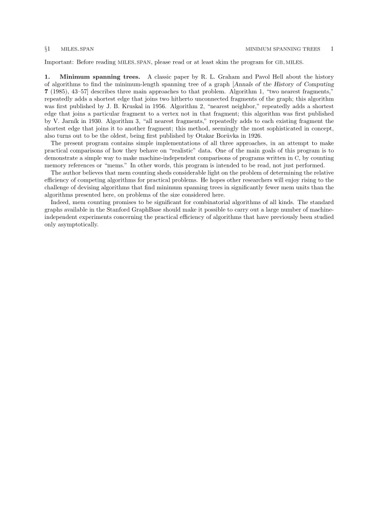
1 1 MILES SPAN MINIMUM SPANNING TREES Important: Before reading MILES SPAN , please read or at least skim the program for GB MILES . 1. Minimum spanning trees. A classic paper by R. L. Graham and Pavol Hell about the history of algorithms
§ 1 1 MILES SPAN MINIMUM SPANNING TREES Important: Before reading MILES SPAN , please read or at least skim the program for GB MILES . 1. Minimum spanning trees. A classic paper by R. L. Graham and Pavol Hell about the history of algorithms to find the minimum-length spanning tree of a graph [ Annals of the History of Computing 7 (1985), 43–57] describes three main approaches to that problem. Algorithm 1, “two nearest fragments,” repeatedly adds a shortest edge that joins two hitherto unconnected fragments of the graph; this algorithm was first published by J. B. Kruskal in 1956. Algorithm 2, “nearest neighbor,” repeatedly adds a shortest edge that joins a particular fragment to a vertex not in that fragment; this algorithm was first published by V. Jarn´ ık in 1930. Algorithm 3, “all nearest fragments,” repeatedly adds to each existing fragment the shortest edge that joins it to another fragment; this method, seemingly the most sophisticated in concept, also turns out to be the oldest, being first published by Otakar Bor˚ uvka in 1926. The present program contains simple implementations of all three approaches, in an attempt to make practical comparisons of how they behave on “realistic” data. One of the main goals of this program is to demonstrate a simple way to make machine-independent comparisons of programs written in C , by counting memory references or “mems.” In other words, this program is intended to be read, not just performed. The author believes that mem counting sheds considerable light on the problem of determining the relative efficiency of competing algorithms for practical problems. He hopes other researchers will enjoy rising to the challenge of devising algorithms that find minimum spanning trees in significantly fewer mem units than the algorithms presented here, on problems of the size considered here. Indeed, mem counting promises to be significant for combinatorial algorithms of all kinds. The standard graphs available in the Stanford GraphBase should make it possible to carry out a large number of machine- independent experiments concerning the practical efficiency of algorithms that have previously been studied only asymptotically.
2 § 2 MINIMUM SPANNING TREES MILES SPAN 2. The graphs we will deal with are produced by the miles subroutine, found in the GB MILES module. As explained there, miles ( n, north weight , west weight , pop weight , 0 , max degree , seed ) produces a graph of n ≤ 128 vertices based on the driving distances between North American cities. By default we take n = 100, north weight = west weight = pop weight = 0, and max degree = 10; this gives billions of different sparse graphs, when different seed values are specified, since a different random number seed generally results in � 128 � the selection of another one of the possible subgraphs. 100 The default parameters can be changed by specifying options on the command line, at least in a UNIX implementation, thereby obtaining a variety of special effects. For example, the value of n can be raised or lowered and/or the graph can be made more or less sparse. The user can bias the selection by ranking cities according to their population and/or position, if nonzero values are given to any of the parameters north weight , west weight , or pop weight . Command-line options −n � number � , −N � number � , −W � number � , −P � number � , −d � number � , and −s � number � are used to specify non-default values of the respective quantities n , north weight , west weight , pop weight , max degree , and seed . If the user specifies a −r option, for example by saying ‘ miles_span −r10 ’, this program will investigate the spanning trees of a series of, say, 10 graphs having consecutive seed values. (This option makes sense only if north weight = west weight = pop weight = 0, because miles chooses the top n cities by weight. The procedure rarely needs to use random numbers to break ties when the weights are nonzero, because cities rarely have exactly the same weight in that case.) The special command-line option −g � filename � overrides all others. It substitutes an external graph previously saved by save graph for the graphs produced by miles . Here is the overall layout of this C program: # include "gb_graph.h" / ∗ the GraphBase data structures ∗ / # include "gb_save.h" / ∗ restore graph ∗ / # include "gb_miles.h" / ∗ the miles routine ∗ / � Preprocessor definitions � � Global variables 3 � � Procedures to be declared early 67 � � Priority queue subroutines 24 � � Subroutines 7 � main ( argc , argv ) int argc ; / ∗ the number of command-line arguments ∗ / char ∗ argv [ ]; / ∗ an array of strings containing those arguments ∗ / { unsigned long n = 100; / ∗ the desired number of vertices ∗ / unsigned long n weight = 0; / ∗ the north weight parameter ∗ / unsigned long w weight = 0; / ∗ the west weight parameter ∗ / unsigned long p weight = 0; / ∗ the pop weight parameter ∗ / unsigned long d = 10; / ∗ the max degree parameter ∗ / long s = 0; / ∗ the random number seed ∗ / unsigned long r = 1; / ∗ the number of repetitions ∗ / char ∗ file name = Λ; / ∗ external graph to be restored ∗ / � Scan the command-line options 4 � ; while ( r −− ) { if ( file name ) g = restore graph ( file name ); else g = miles ( n, n weight , w weight , p weight , 0 L , d, s ); if ( g ≡ Λ ∨ g �n ≤ 1) { fprintf ( stderr , "Sorry, � can’t � create � the � graph! � (error � code � %ld)\n" , panic code ); return − 1; / ∗ error code 0 means the graph is too small ∗ / } � Report the number of mems needed to compute a minimum spanning tree of g by various algorithms 5 � ; gb recycle ( g );
§ 2 3 MILES SPAN MINIMUM SPANNING TREES s ++ ; / ∗ increase the seed value ∗ / } return 0; / ∗ normal exit ∗ / } 3. � Global variables 3 � ≡ Graph ∗ g ; / ∗ the graph we will work on ∗ / See also sections 6, 10, 13, 19, 23, 31, 37, 57, and 68. This code is used in section 2. 4. � Scan the command-line options 4 � ≡ while ( −− argc ) { if ( sscanf ( argv [ argc ] , "−n%lu" , & n ) ≡ 1) ; else if ( sscanf ( argv [ argc ] , "−N%lu" , & n weight ) ≡ 1) ; else if ( sscanf ( argv [ argc ] , "−W%lu" , & w weight ) ≡ 1) ; else if ( sscanf ( argv [ argc ] , "−P%lu" , & p weight ) ≡ 1) ; else if ( sscanf ( argv [ argc ] , "−d%lu" , & d ) ≡ 1) ; else if ( sscanf ( argv [ argc ] , "−r%lu" , & r ) ≡ 1) ; else if ( sscanf ( argv [ argc ] , "−s%ld" , & s ) ≡ 1) ; else if ( strcmp ( argv [ argc ] , "−v" ) ≡ 0) verbose = 1; else if ( strncmp ( argv [ argc ] , "−g" , 2) ≡ 0) file name = argv [ argc ] + 2; else { fprintf ( stderr , "Usage: � %s � [−nN][−dN][−rN][−sN][−NN][−WN][−PN][−v][−gfoo]\n" , argv [0]); return − 2; } } if ( file name ) r = 1; This code is used in section 2.
Recommend
More recommend
Explore More Topics
Stay informed with curated content and fresh updates.
