0.1 Naive formulation of PageRank In general, PageRank is a way to - PDF document

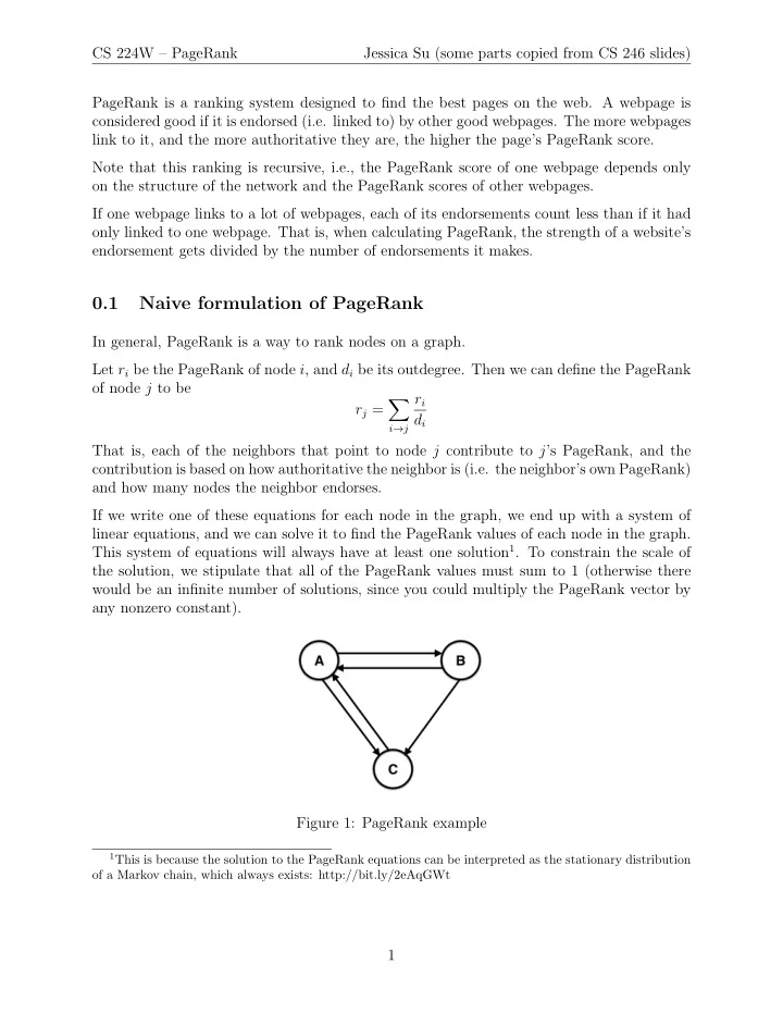
CS 224W – PageRank Jessica Su (some parts copied from CS 246 slides) PageRank is a ranking system designed to find the best pages on the web. A webpage is considered good if it is endorsed (i.e. linked to) by other good webpages. The more webpages link to it, and the more authoritative they are, the higher the page’s PageRank score. Note that this ranking is recursive, i.e., the PageRank score of one webpage depends only on the structure of the network and the PageRank scores of other webpages. If one webpage links to a lot of webpages, each of its endorsements count less than if it had only linked to one webpage. That is, when calculating PageRank, the strength of a website’s endorsement gets divided by the number of endorsements it makes. 0.1 Naive formulation of PageRank In general, PageRank is a way to rank nodes on a graph. Let r i be the PageRank of node i , and d i be its outdegree. Then we can define the PageRank of node j to be r i � r j = d i i → j That is, each of the neighbors that point to node j contribute to j ’s PageRank, and the contribution is based on how authoritative the neighbor is (i.e. the neighbor’s own PageRank) and how many nodes the neighbor endorses. If we write one of these equations for each node in the graph, we end up with a system of linear equations, and we can solve it to find the PageRank values of each node in the graph. This system of equations will always have at least one solution 1 . To constrain the scale of the solution, we stipulate that all of the PageRank values must sum to 1 (otherwise there would be an infinite number of solutions, since you could multiply the PageRank vector by any nonzero constant). Figure 1: PageRank example 1 This is because the solution to the PageRank equations can be interpreted as the stationary distribution of a Markov chain, which always exists: http://bit.ly/2eAqGWt 1

CS 224W – PageRank Jessica Su (some parts copied from CS 246 slides) 0.1.1 Example The PageRank equations for the graph in Figure 1 are r A = r B / 2 + r C r B = r A / 2 r C = r A / 2 + r B / 2 (In addition, we enforce the constraint that r A + r B + r C = 1.) 0.2 Matrix representation We can keep all the PageRank values in a vector   r 1 r 2   r = .   .  .    r n In which case the PageRank equations become r = M r where M is a “weighted adjacency matrix” that contains the structure of the network. Specifically, we have � 1 if j links to i d j M ij = 0 otherwise Note that the columns of M must sum to 1 (so M is a “column stochastic matrix”). 0.2.1 Example We can write the previous example in the form r = M r by writing   0 1 / 2 1 M = 1 / 2 0 0   1 / 2 1 / 2 0 and   r A r = r B   r C 2

CS 224W – PageRank Jessica Su (some parts copied from CS 246 slides) 0.3 Eigenvalue interpretation Since r = M r , we know that assuming r exists, it must be an eigenvector of the stochastic web matrix M (where the eigenvalue is 1). We show that specifically, it must be the principal eigenvector of M (i.e. the eigenvector corresponding to the eigenvalue of largest magnitude). Proof: Recall the definition of the L 1 vector norm: n � || x || 1 = | x i | i =1 Using the L 1 vector norm, we can define an induced L 1 matrix norm, as follows: || A x || 1 || A || 1 = max || x || 1 x � =0; x ∈ R n It follows directly from the definition that || A x || 1 ≤ || A || 1 || x || 1 for any matrix A and vector x . However, this doesn’t help much if we can’t evaluate || A || 1 . Fortunately, there is an alternate, more convenient formula for evaluating the induced L 1 matrix norm: 2 n � || A || 1 = max | A ij | j i =1 That is, the induced L 1 matrix norm of a matrix A is the sum of the entries in the “largest” column. How does this relate to the eigenvalues? Suppose that x is an eigenvector of M . We know that || M x || 1 ≤ || M || 1 || x || 1 . Since M is a column-stochastic matrix, all of its columns must sum to 1, so the convenient formula for || M || 1 gives us 1. Therefore || M x || 1 ≤ || x || 1 . However, the eigenvalue formula says that M x = λ x , and taking norms on both sides, we get || M x || 1 = λ || x || 1 . Therefore, λ must be less than or equal to 1. 0.4 Power iteration One way to solve for r is by using power iteration . The idea is we start by setting r = [1 /n, 1 /n, . . . , 1 /n ] T . Then we keep multiplying it by M over and over again until we reach a steady state (i.e. the value of r doesn’t change). This will give us a solution to r = M r . Formally, we let r (0) = [1 /n, 1 /n, . . . , 1 /n ] T , then we iteratively compute r ( t +1) = M r ( t ) for each t until | r ( t +1) − r ( t ) | 1 < ǫ . (Note that | x | 1 = � i | x i | is the L 1 norm.) Then r ( t +1) is our estimate for the PageRank values. 2 http://pages.cs.wisc.edu/ sifakis/courses/cs412-s13/lecture notes/CS412 19 Mar 2013.pdf 3

CS 224W – PageRank Jessica Su (some parts copied from CS 246 slides) 0.4.1 Why power iteration converges to a principal eigenvector of the matrix M We claim that the sequence r (0) , r (1) , r (2) , . . . converges to the principal eigenvector of M (which are the PageRank values). Proof: Assume that the n -by- n matrix M has n linearly independent eigenvectors x 1 , . . . , x n , with corresponding eigenvalues 1 = λ 1 > λ 2 > · · · > λ n . (If this is not true, the proof is harder, and it can be found on Wikipedia. 3 ) Then the vectors x 1 , . . . , x n form a basis of R n , so we can write r (0) = c 1 x 1 + c 2 x 2 + · · · + c n x n Since M is a linear operator, we have M r (0) = M ( c 1 x 1 + c 2 x 2 + · · · + c n x n ) = c 1 ( M x 1 ) + c 2 ( M x 2 ) + · · · + c n ( M x n ) = c 1 ( λ 1 x 1 ) + c 2 ( λ 2 x 2 ) + · · · + c n ( λ n x n ) By the same logic, M k r (0) = c 1 ( λ k 1 x 1 ) + c 2 ( λ k 2 x 2 ) + · · · + c n ( λ k n x n ) Since λ 1 = 1 and λ 2 , . . . , λ n are all less than 1, we get r ( k ) → c 1 x 1 as k → ∞ . That is, r approaches the dominant eigenvector of M . 0.5 Markov chain interpretation One way to interpret PageRank is as follows. Imagine you are a web surfer who spends an infinite amount of time on the internet (which isn’t too far from reality). At any time t , you are at a page i , and at time t + 1, you follow an out-link from i uniformly at random, ending up at one of i ’s neighbors. Let p ( t ) be the vector whose i th coordinate is the probability that the surfer is at page i at time t . ( p ( t ) is a probability distribution over pages, and its entries sum to 1.) Recall that M ij is the probability of moving from node j to node i , given that you are already on node j , and p j ( t ) is the probability that you are on node j at time t . Therefore, for each node i , we have p i ( t + 1) = M i 1 p 1 ( t ) + M i 2 p 2 ( t ) + · · · + M in p n ( t ) 3 https://en.wikipedia.org/wiki/Power iteration 4

CS 224W – PageRank Jessica Su (some parts copied from CS 246 slides) Which means p ( t + 1) = M p ( t ) If the random walk ever reaches a state where p ( t + 1) = p ( t ), then p ( t ) is a stationary distribution for this random walk. Recall that the PageRank vector r = M r . So the PageRank vector r is a stationary distribution for the random walk! For graphs that satisfy certain conditions, this stationary distribution is unique, and will eventually be reached regardless of the initial probability distribution at time t = 0. 0.6 Final formulation of PageRank One of the problems with the way we formulated PageRank is that some nodes might not have any out-links. In this case, the random web surfer gets stuck at a “dead end” and can’t visit any more pages, ruining our plans. Similarly, the web surfer may get stuck in a “spider trap” of pages where all the links only point to pages inside the spider trap. In that case, the pages in the spider trap eventually absorb all the PageRank, leaving none of the PageRank for other pages. In order to deal with the spider trap problem, we add an escape route. We say that with probability β (which is usually about 0 . 8 or 0 . 9), the web surfer follows an out-link at random, but with probability 1 − β , he jumps to some random webpage. In the case of a dead end, the web surfer jumps to a random webpage 100% of the time. With this modification, the new PageRank equation becomes β r i + (1 − β )1 � r j = d i n i → j where d i is the outdegree of node i . (This formulation assumes there are no dead ends.) Similar to our previous matrix M , we can define a new matrix � 1 � A = βM + (1 − β ) n n × n that reflects the new transition probabilities. Now we just have to solve the equation r = A r instead of r = M r , and we can do that using power iteration. 1 References “CS 246 Lecture 9: PageRank (2014).” http://stanford.io/2fDoChT “Markov Chains.” MIT OpenCourseWare, http://bit.ly/2eAqGWt 5

CS 224W – PageRank Jessica Su (some parts copied from CS 246 slides) “CS 412 Lecture Notes: Linear Algebra.” http://bit.ly/2fDyZ3d “Power Iteration.” https://en.wikipedia.org/wiki/Power_iteration 6